Oct 18, 2025
Making LLMs Efficient in Production
A practical journey to deploy faster, cheaper LLM/transformer models using distillation, quantization, and ONNX Runtime—no PhD required.
The heavy model in your backpack
Ever tried to stuff your entire wardrobe into a single carry-on? That's what deploying a large language model can feel like. In Transformers: Simple Yet Wildly Versatile I showed how a simple attention-only architecture conquered translation, vision and even diffusion models. But there's a catch: the very models that write essays and fix code can also be unwieldy when you try to ship them. A vanilla BERT base checkpoint tips the scales at over 400 MB and takes tens of milliseconds to answer a single query. When you're serving thousands of requests per second, those delays add up.
What I optimize in this post: a BERT-class transformer (encoder-only) fine-tuned for intent classification. I’ll use “LLM” broadly when talking about production impact, and “transformer/BERT” when referring to the exact model and code.
Why speed matters in practice (not theory):
- Throughput: Faster models = more requests/sec per instance
- Cost: Same hardware handles more traffic or the same traffic at lower cost
- Memory: Smaller checkpoints run more workers per machine
- UX: Lower latency → snappier responses and more headroom for spikes
In this post I’ll take you on a practical journey to lighten that load. We’ll start with shipping a full BERT into production—and gradually unpack tricks like distillation, quantization, and ONNX Runtime.
Baseline BERT
My journey began with a simple question: How fast and accurate is a plain BERT? I wrote a small helper to benchmark size, latency and accuracy. Environment: CPU inference on a modern x86 instance; batch size 1; latency is per-request average.
class PerformanceBenchmark: def __init__(self, model_name_or_path, task='text-classification'): self.pipeline = pipeline(task=task, model=model_name_or_path) def benchmark(self, test_dataset): # Version-proof model size in MB model_size = sum(p.numel() * p.element_size() for p in self.pipeline.model.parameters()) / (1024**2) latencies, correct = [], 0 for item in test_dataset: start = time.time() pred = self.pipeline(item['text'])[0]['label'] latencies.append((time.time() - start) * 1000) correct += (pred == item['intent']) return { 'model_size': model_size, 'avg_latency': float(np.mean(latencies)), 'accuracy': correct / len(test_dataset) }
Results (CLINC OOS intent classification):
| Model | Size (MB) | Latency (ms) | Accuracy (%) |
|---|---|---|---|
| BERT | ~418 | ~40 | 86.7 |
Capacity & cost framing (40 ms):
- To serve 1,000 req/s: ~40 parallel workers
- Memory: 418 MB/worker limits packing density per machine
First stop: off-the-shelf distillation
What it is: Distillation is model compression via teacher–student training. A smaller student learns to imitate a larger teacher—not just the teacher’s final labels, but its confidence profile over classes.
How it works (practically): I load a strong teacher (BERT fine-tuned on CLINC) and a compact student (DistilBERT). During training, I optimize two things at once:
- the usual cross-entropy on ground-truth labels, and
- a KL-divergence term that pushes the student’s logits toward the teacher’s softened logits (temperature > 1). The temperature spreads out the teacher’s probabilities so the student can learn relative preferences (“A is twice as likely as B”) rather than only hard labels. A mixing weight alpha controls how much to trust teacher vs. labels.
Why it helps: Soft targets contain extra information that hard labels throw away. The student inherits some of the teacher’s generalization while using fewer parameters.
I tried the ready-made checkpoint transformersbook/distilbert-base-uncased-finetuned-clinc.
| Model | Size (MB) | Latency (ms) | Accuracy (%) |
|---|---|---|---|
| DistilBERT (HF) | ~250 | ~22 | 85.5 |
Capacity & cost framing (22 ms):
- To serve 1,000 req/s: ~22 workers (≈45% fewer than BERT)
- Memory: 250 MB → ~1.6× more workers per machine vs BERT
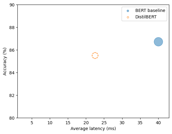
To visualise the progress, I plotted average latency versus accuracy, using bubble size to encode model size. The blue bubble (BERT) sits far to the right—big and slow. The orange bubble (DistilBERT) shifts left on latency while staying reasonably high on accuracy:
A quick win—but could a student I trained do even better?
Distillation: teaching my own student
What I change vs. off-the-shelf: I keep the teacher–student recipe but tune the blend (alpha) and temperature for my data, and optionally unfreeze more layers or train a bit longer. I also monitor which classes the student struggles with and adjust the loss weights if needed.
Why it works better: Off-the-shelf students are generic. A short, targeted run on your actual distribution lets the student specialize. Think of it like a chef showing the sous-chef your kitchen’s menu and rush-hour patterns—not just cooking in theory.
distil_config = DistillationConfig( teacher_model=teacher_model, student_model=AutoModelForSequenceClassification.from_pretrained( 'distilbert-base-uncased', num_labels=num_labels), alpha=0.5, temperature=2.0, epochs=3, learning_rate=5e-5, ) trainer = DistillationTrainer(distil_config) trainer.train(train_dataset) metrics = trainer.evaluate(test_dataset)
| Model | Size (MB) | Latency (ms) | Accuracy (%) |
|---|---|---|---|
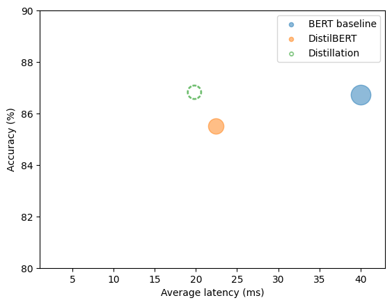
| Custom Distilled | ~250 | ~20 | 86.8 |
Capacity & cost framing (20 ms):
- To serve 1,000 req/s: ~20 workers (≈2× cheaper than baseline at same traffic)
Deep compression: dynamic quantization
What it is: Quantization reduces numeric precision to make math cheaper. Instead of 32-bit floats everywhere, we represent weights (and sometimes activations) as 8-bit integers and keep per-tensor (or per-channel) scales/zero-points to map back and forth.
How it works (in practice): With dynamic quantization in PyTorch, I wrap the model and tell it to quantize Linear layers at runtime. The weights are stored in INT8; activations are observed dynamically and quantized on the fly. The core attention math still behaves the same logically—just with lighter arithmetic and less memory bandwidth.
Why it helps: Transformers are dense-matmul heavy. Shrinking weights/activations cuts memory traffic and lets CPUs use faster integer kernels. As a side effect, the small quantization noise can act like regularization—the model sometimes gets a tiny accuracy bump.
quantized_model = torch.quantization.quantize_dynamic( distilled_model, {nn.Linear}, dtype=torch.qint8 )
| Model | Size (MB) | Latency (ms) | Accuracy (%) |
|---|---|---|---|
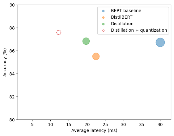
| Quantized | ~132 | ~12 | 87.6 |
Capacity & cost framing (12 ms):
- To serve 1,000 req/s: ~12 workers (~3.3× fewer than baseline)
- Memory: 132 MB → ~3× more workers per machine vs BERT
A small surprise: When the quantized model slightly outperformed the original on accuracy, I thought I’d miscalculated. It wasn’t a bug—quantization can act as a mild regularizer.
Going further: ONNX Runtime and hardware-accelerated inference
What it is: ONNX is a portable model format; ONNX Runtime (ORT) is a high-performance engine with optimized kernels for CPUs/GPUs/accelerators.
How it works (end-to-end):
- Export the trained PyTorch model to ONNX with dynamic axes (so batch can vary).
- Load it in ORT and select providers (e.g.,
CPUExecutionProvider, CUDA, etc.). - Optionally run ORT’s quantization pass to get INT8 benefits on top of its kernels.
- Deploy the single ONNX artifact broadly—handy when your fleet spans multiple hardware types.
Why it helps: Even without changing the model, a better executor wins. ORT fuses ops, picks faster kernels, and reduces framework overhead. On CPUs, pairing ORT with quantization compounds the gains.
# Export to ONNX (CPU path) inputs = tokenizer('hello world', return_tensors='pt') torch.onnx.export( distilled_model, (inputs['input_ids'], inputs['attention_mask']), 'distilled.onnx', input_names=['input_ids','attention_mask'], output_names=['logits'], dynamic_axes={'input_ids': {0: 'batch'}, 'attention_mask': {0: 'batch'}}, opset_version=16, ) ort_session = ort.InferenceSession('distilled.onnx', providers=['CPUExecutionProvider'])
| Model | Size (MB) | Latency (ms) | Accuracy (%) |
|---|---|---|---|
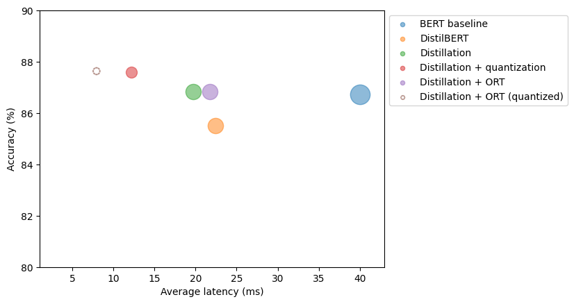
| ORT (quantized) | ~132 | ~8 | ~87.7 |
Capacity & cost framing (8 ms):
- To serve 1,000 req/s: ~8 workers → ~5× fewer instances vs 40 ms baseline
- Memory: small artifact + ORT quantization → dense packing and better autoscaling headroom
Conclusion: the short playbook (no silver bullets)
Pick by constraint, then iterate:
- Quick win / low effort: start with an off-the-shelf distilled model.
- Accuracy + speed: run DIY distillation (teacher–student with temperature + alpha).
- Edge/CPU or memory-bound: apply dynamic quantization first.
- Cross-platform & kernel speed: export to ONNX and run with ONNX Runtime (+ ORT quantization).
- Chasing the last mile: combine them (distillation → quantization → ORT), then consider structured pruning and serving-stack tweaks.
One-glance summary
| Model | Size (MB) | Latency (ms) | Accuracy (%) | Speedup vs BERT |
|---|---|---|---|---|
| BERT | 418 | 40 | 86.7 | 1.0× |
| DistilBERT (HF) | 250 | 22 | 85.5 | 1.8× |
| Custom Distilled | 250 | 20 | 86.8 | 2.0× |
| Quantized | 132 | 12 | 87.6 | 3.3× |
| ORT Quantized | 132 | 8 | 87.7 | 5.0× |
Shout-out & further reading
A huge shout-out to Lewis Tunstall, Leandro von Werra, and Thomas Wolf—much of the way I think about distillation, quantization, and practical deployment comes from their book, Natural Language Processing with Transformers. If you're hungry for a deeper, hands-on tour, start here:
Natural Language Processing with Transformers (Revised Edition) — Read/buy on O'Reilly Media.